信号博弈是经济学和决策理论中的一个重要概念,它旨在解释如何在存在信息不对称的情况下,通过信号传递和反应函数的相互作用,实现均衡。信息不对称是指参与博弈的各方所拥有的信息不同,这可能导致不公平的结果。信号传递是指通过某种行为或信号,传递信息给其他参与方,以改善信息的对称性,反应函数是指根据接收到的信号,参与者做出的最佳反应决策。信号博弈的应用广泛,如劳动力市场、保险市场、金融市场等,有助于解决信息不对称带来的问题,提高市场效率。
一、信号传递
孔雀开屏信号。孔雀寓意着聪明、善良、自由、和平,一般孔雀象征着吉祥、幸福、高洁华贵,同时也表示长寿之意。孔雀是百鸟之王,是吉祥鸟,因此,孔雀受到了广大人民的喜爱与青睐,其观赏价值也是比较的高。孔雀是一种吉祥鸟,它体态优美,丹口玄目,细劲隆胸。而且也是最善良、最聪明、最爱自由与和平的鸟,是吉祥幸福的象征,孔雀也可以看为是绶带鸟绶与寿谐音,表示长寿之意。在希腊神话中,孔雀更是象征着赫拉女神。它能够给人带来好运,不断激励着人去前进。
产品质量信号:假设有一家公司生产某种产品,但消费者无法直接判断产品的质量。公司可以通过选择不同的包装、广告宣传和保修政策来传递关于产品质量的信号。例如,一个公司可能选择使用高质量的包装和昂贵的广告来暗示其产品的高质量,以吸引更多消费者购买。
教育水平信号:在劳动市场中,个体的教育水平往往是一种信号,用于向潜在雇主传达其技能和能力水平。人们可能会选择接受更高水平的教育,部分原因是为了向未来的雇主展示其能力,从而增加就业机会。
金融市场信号:在金融市场中,公司可以通过发布财务报表、举办电话会议等方式来传递有关其业务状况和未来前景的信号。这些信号可能影响投资者的决策,从而影响股价和市场走势。
信号博弈”是研究具有信息传递特征的信号机制的一般非完全信息动态博弈模型。信号博弈的基本特征是两个(或两类,每类又有若干个)博弈方,分别称为信号发出方(Sender)和信号接收方(Receiver),他们先后各选择一次行为,其中信号接收方具有不完全信息,但他们可以从信号发出方的行为中获得部分信息,信号发出方的行为对信号接收方来说,好像是一种(以某种方式)反映其有关得益信息的信号。这也正是这类博弈被称为“信号博弈”的原因。
由于信号博弈也是动态贝叶斯博弈,因此也可以通过海萨尼转换直接表示成完全但不完美信息动态博弈。设自然(博弈方0)先按特定的概率分布从信号发出方的类型空间中为发出方随机选择一个类型,并将该类型告诉发出方(即发出一个信号);然后是接收方在自己的行为空间中选择一个行为(也称发出一个信号);最后接收方根据发出方的行为选择自己的行为。如果我们用\(S\)表示信号发出方,用\(R\)表示信号接收方,用 \(T=\{t_{1},...,t_{I}\}\)表示\(S\)的类型空间,用\(M=\{m_{1},...,m_{J}\}\) 表示\(S\)的行为空间,或者称信号空间,用\(a=\{a_{1},...,a_{K}\}\)表示 \(R\)的行为空间,用\(u_{s}\)和\(u_{R}\)分别表示\(S\)和\(R\)的得益,并且自然为\(S\)选择类型的概率分布为$${p(t_{1}),...,p(t_{i})}$$。因此,信号博奔的时间顺序可表示为:
(1)博弈方0(自然)以概率\(p(t_{i})\)从可行的类型集\(T\)中为发送者 \(S\)选择类型\(t_{i}\),并让\(S\)知道,这里对所有的\(i\),\(p(t_{i})>0\) ,且 \(p(t_{1}),...,p(t_{I})=1\)。
(2)发送者\(S\)观测到\(t_{i}\)后,从可行的信号集\(M\)中选择行为 \(m_{j}\) 。
(3)接收者\(R\)看到\(m_{j}\),(但不能观测到\(t_{i}\))后从可行的行为空间中选择行为\(a_{k}\)。
(4)发送者\(S\)和接收者\(R\)的得益\(u_{S}\)和\(u_{R}\)都取决于\(t_{i}\) 、\(m_{j}\)和\(a_{k}\)。
注意 \(T\)、\(M\)和\(A\)既可以是离散空间,也可以是连续空间。
3.1 信号博弈完美贝叶斯纳什均衡
这里,我们简单地将类型空间、可行信号集与可行行动集定义为有限集合,在实际应用中,它们常常表现为连续的区间,显然,此时可行信号集依赖于类型空间,而可行行动集则依赖于发送者发出的信号。这是一个简单的信号博弈,其中\(N\)表示自然,\(T=\{t_{1},t_{2}\}\), \(M=\{m_{1},m_{2}\}\),\(A=\{a_{1},a_{2}\}\) ,图中\(p\) 及\(1−p\)表示自然选择类型时的概率分布。
在信号博弈中,发送者的纯策略是根据自然抽取的可能类型来选取相应的信号,因此,信号可视作类型\(t\)的函数\(m(t_{i})\)。接收者的纯策略是信号的函数\(a(m_{j})\),即根据观察到的发送者发出的信号确定自已的行动。在下图的信号博弈中,发送者 \(S\)与接收者\(R\)各有四个纯策略。
发送者的纯策略:
发送者\(S\)的策略1,记为\(S(1)\):若自然抽取\(t_{1}\),选择 \(m_{1}\) ;若自然抽取\(t_{2}\),则选择\(m_{1}\);
发送者\(S\)的策略2,记为\(S(2)\):若自然抽取\(t_{1}\),选择 \(m_{1}\);若自然抽取\(t_{2}\),则选择 \(m_{2}\);
发送者\(S\)的策略3,记为\(S(3)\):若自然抽取\(t_{1}\),选择 \(m_{2}\);若自然抽取\(t_{2}\),则选择 \(m_{1}\);
发送者\(S\)的策略4,记为\(S(4)\):若自然抽取\(t_{1}\),选择 \(m_{2}\);若自然抽取\(t_{2}\),则选择 \(m_{2}\);
接收者的纯策略:
接收者\(R\)的策略1,记为\(R(1)\):若\(S\)发出\(m_{1}\),选择 \(a_{1}\);若 \(S\)发出\(m_{2}\),则选择\(a_{1}\);
接收者\(R\)的策略2,记为\(R(2)\):若\(S\)发出\(m_{1}\),选择 \(a_{1}\);若 \(S\)发出\(m_{2}\),则选择\(a_{2}\);
接收者\(R\)的策略3,记为\(R(3)\):若\(S\)发出\(m_{1}\),选择 \(a_{2}\);若 \(S\)发出\(m_{2}\),则选择\(a_{1}\);
接收者\(R\)的策略4,记为\(R(4)\):若\(S\)发出\(m_{1}\),选择 \(a_{2}\);若 \(S\)发出\(m_{2}\),则选择\(a_{2}\);
发送者\(S\)的纯策略中的\(S(1)\)与\(S(4)\)有一个特点,对于“自然”抽取的不同类型,\(S\)选择相同的信号,我们称具有这类特点的策略称为混同(Pooling)策略。对于\(S(2)\)与\(S(3)\),由于对不同的类型发出不同的信号,称为分离(Separating)策略。由于在这个简单情况中各种集合只有两个元素,因此博弈方的纯策略也只有混同与分离这两种,假如类型空间的元素多于两个,那么就有部分混同或准分离策略。实际上各种类型分为不同的组,对于给定的类型组中所有类型,发送者发出相同的信号:而对于不同组的类型则发生不同的信号。
在下图的博弈中当自然抽取\(t_{2}\),\(S\)在\(m_{1}\)和\(m_{2}\)这两个信号中随机选择,这样的策略称为杂合策略,这里只讨论纯策略。

由于信号博弈可以表示为完全但不完美信息动态博弈的形式,我们就可以利用精练叶斯均衡对它们进行分析。信号发送者在选择信号时知道博弈全过程,这一选择发生于单节信息集(对自然可能抽取的每一种类型都存在一个这样的信息集)。因此要求1在应用于发送者时就无需附加任何条件;如果接收者在不知道发送者类型的条件下观察到发送者的信号并选择行动,也就是说接收者的选择处于一个非单点的信息集(对发送者可能选择的每一种信号都存在一个这样的信息集,而且每一个这样的信息集中,各有一个节点对应于自然可能抽取的每一种类型)。下面我们把关于精练贝叶斯均衡要求1至要求4的事述转化为信号博弈中对精练贝叶斯均衡的要求。根据信号博弈的特点,其精练贝叶均衡的条件是:
信号要求1:(把要求1应用于 \(R\) ) 信号接收者 \(R\) 在观察到信号发出者 \(S\) 的信号后,必须有关于 \(S\) 的类型的推断,即 \(S\) 选择 \(m_j\) 时, \(S\) 是每种类型 \(t_i\) 的概率分布 \(p\left(t_i \mid m_j\right) \cdot p\left(t_i \mid m_j\right) \geq 0\) ,且 \(\sum p\left(t_i \mid m_j\right)=1\) 。
给出了信号发出方 \(S\) 信号和信号接收方 \(R\) 的推断后,再描述 \(R\) 的最优行为便十分简单。
信号要求2R:(把要求2应用于 \(R\) ) 给定 \(R\) 的判断 \(p\left(t_i \mid m_j\right)\) 和 \(S\) 的信号 \(m_j , R\) 的行为 \(a^*\left(m_j\right)\) 必须使 \(R\) 的期望得益最大,即 \(a^*\left(m_j\right)\) 是最大化问题
的解。
信号要求2S:(把要求2应用于 \(S\) ) 给定 \(R\) 的策略 \(a^*\left(m_j\right)\) 时, \(S\) 的选择 \(m^*\left(t_i\right)\) 必须使 \(S\) 的 得益最大,即 \(m^*\left(t_i\right)\) 是最大化问题
的解。
信号要求3:(把要求3、4应用于 \(R\) ) 对每个 \(m_j \in M\) ,如果存在 \(t_i \in T\) 使得 \(m^*\left(t_i\right)=m_j\) ,则 \(R\) 在对应于 \(m_j\) 的信息集处的判断必须符合 \(S\) 的策略和贝叶斯法则。即使 不存在 \(t_i \in T\) 使 \(m^*\left(t_i\right)=m_j , R\) 在 \(m_j\) 对应的信息集处的判断也仍要符合 \(S\) 的策略和贝 叶斯法则。即:
因为上述双方策略都是纯策略,因此是纯策略完美贝叶斯均衡。
3.2 企业并购中的信号传递模型
在企业并购过程中,并购双方对于并购信息的掌握是不对称的,并购企业总是处于有息不利的地位。目标企业的管理水平、产品开发能力、机构效率、投资政策、财务政策未来生产经营情况等因素将会影响企业未来的价值,但并购企业并不完全了解这些信息,因此,企业并购中存在信息不对称现象。
基本假设
(1)假定有两个时期\(T_{1}\)和\(T_{2}\),两个参与人(并购企业与目标企业)。
(2)假定目标企业在\(T_{2}\)时期的价值\(v\)服从\([0,\theta]\)上的均匀分布,目标企业知道\(\theta\) 的确切值;高质量的目标企业价值大,低质量的目标企业价值小;并购企业不知道\(\theta\),但知道目标企业属于 \(\theta\)的先验概率\(p(\theta)\)。
(3)目标企业根据自己的类型向并购企业传递信号\(x\) (我们假定目标企业发出的信号\(x\)能真实地反映目标企业的类型,不存在欺诈现象)。并购企业能从信号中推断出目标企业的预期价值水平,也就是目标企业会根据自己的真实情况向并购企业传递信息,而不是传递虚假信息。若并购企业为知情者,则其推断出目标企业的预期价值水平为 \(\beta\theta(x)\),若并购企业为未知情者,则其推断出目标企业的预期价值水平为 \(\theta(x)/2\),其中,\(x\)为目标企业发出的信号,\(\theta(x)\)为未知情的并购企业依据目标企业的信号\(x\)推断出的目标企业的最大预期价值水平。
(4)并购企业不知道目标企业的类型\(\theta\),只知道目标企业属于 \(\theta\)的概率分布\(p(\theta)\),则目标企业向并购企业发出信号\(x\) 时,并购企业根据目标企业发出的信号\(x\)推断出目标企业的预期价值水平为 \(\bar{v}(x)=\theta(x)/2\)。
(5)对于目标企业而言,其目标是最大化\(T_{1}\)时企业的价值和 \(T_{2}\) 时的预期价值水平的加权平均:
其中,\(\bar{v_{0}}(x)\) 是目标企业发出信号\(x\)时,目标企业在 \(T_{1}\)时期的价值:\(\omega\) 是\(T_{2}\)时期目标企业预期价值的权重, \(0\leq \omega \leq 1\);\(p_{s}\)为目标企业在寿命期内经营成功的概率;\(p_{1}=x/\theta\leq 1\),是目标企业在寿命期内经营失败的概率, \(p_{2}\) 为目标企业在寿命期内经营一般的概率;\(L_{1}\)是目标企业在寿合期内完全失败时道受的破产惩罚,\(L_{1} \geq 0\):\(L_{2}\)是目标企业经营一般时企业的价值, \(L_{2} \geq 0\)。
信号博弈过程
(1)“自然”选释目标企业的类型,目标金业在了解到自己的类型后,向并购企业发出关于自身企业的产品质量、投资及财务状况等方面的信号\(x\)。
(2)并购企业在观察到目标企业发出的信号\(x\)后,依据贝叶斯法则对其先验概率\(p(\theta)\)进行修正,得出后验概率$\tilde{p}\left( \theta _{i}/x_{i}\right)$,并据此判断目标企业的预期价值水平 \(\bar{v}(x)\)。
(3)目标企业知道并购企业对其发出信号的反应,因而发出最优信号值 \(x^{*}\),使自身的效用函数最大,即通过求\(max\ u(x,\bar{v}(x),\theta)\),得出 \(x\)的最优值\(x^{\ast}\)。
完美贝叶斯纳什均衡
在信息不完全条件下,并购企业不能直接观察到目标企业的类型,因而对目标企业价值的判断只能根据所观察到的目标企业的信号\(x\)而定,此时,精练贝叶斯均衡满足:
(1)目标企业发出信号\(x\);
(2)并购企业接收到的信号\(x\)得出后验概率\(\tilde{p}=\tilde{p}\left( \theta/x\right)\),并确定对目标企业预期价值水平的评估为 \(\bar{v}(x)\),使得:
①基于目标企业的信念,给定并购企业对信号\(x\)的反应,假定目标企业的目标是最大化\(T_{1}\)时的价值和 \(T_{2}\)时的预期价值水平的加权平均,即:
②从并购企业的角度来看,并购企业对于目标企业发出信号\(x\)的反应,其目的是最大化自己的效用函数\(u_{A}\)。
③ \(\tilde{p}=\tilde{p}\left(\theta /x \right) =\frac{p\ \left( x/\theta \right) p\left( \theta \right) }{\tilde{p}\left( x\right)}\)
均衡结果分析
根据信号博弈的顺序,当目标企业选择信号\(x\)时,将预测到并购企业将据此估计目标企业的价值水平\(\bar{v}(x)=\theta(x)/2\),即并购企业认为目标企业属于类型\(\theta\)的期望是\(\theta(x)\)。考虑分离均衡:
有:
根据(2)式可以看出,价值水平 \(\theta\) 越高的目标企业,其失败的可能性越小,将 \(\bar{v}(x)=\theta(x) / 2\) 代人 (1) 式,有:
对 (3) 式求导,得一阶条件:
出现均衡时,并购企业能从目标企业发出的信号 \(x\) 正确的推断出 \(\theta\) ,即如果 \(x(\theta)\) 是属于类型 \(\theta\) 的目标企业的最好适择,则 \(\theta(x(\theta))=\theta\) ,所以 \(\frac{\partial \theta}{\partial x}=\left(\frac{\partial x}{\partial \theta}\right)^{-1}\) ,将其代入 (4) 式得:
求解 (5) 式得:
(6) 式为目标企业经背者的均衡策略,将 \(\bar{v}(x)=\theta(x) / 2\) 代人 (6) 式,可以得到目标企线的 价值水平表达式如 (7) 式所示:
根据 (7) 式可以看出,目标企业的质量越高,价值就越大;虽然并购企业不能直接观察到目标企业的准确信息,但可以通过分析目标企业发出的信号 \(x\) 来判断目标企业真实的价值水平,从而做出正确的并购决策。
二、MBA信号博弈
Education Signaling: The MBA Game
This section analyzes a very simple version of an education signaling game in the spirit of Spence’s work that sheds some light on the signaling value of education. To focus attention on the signaling value of education, we will ignore any productive value that education may provide. That is, we assume that a person learns nothing productive from education but has to “suffer” the loss of time and the hard work of studying to get a diploma, in this case an MBA degree.1 The game proceeds in the following steps:
- Nature chooses player 1's skill (productivity at work), which can be high \((H)\) or low \((L)\), and only player 1 knows his skill. Thus his type set is \(\Theta=\{H, L\}\). The probability that player 1's type is \(H\) is given by \(\operatorname{Pr}\{\theta=H\}=p>0\), and it is common knowledge that this is Nature's prior distribution.
- After player 1 learns his type, he can choose whether to get an MBA degree \((D)\) or be content with his undergraduate-level degree \((U)\), so that his action set is \(A_1=\{D, U\}\). Getting an MBA requires some effort that is type dependent. Player 1 incurs a private cost \(c_\theta\) if he gets an MBA, and a cost of 0 if he does not. We assume that high-skilled types find it easier to study, captured by the assumption that \(c_H<c_L\). We assume in particular that \(c_H=2\) and \(c_L=5\).
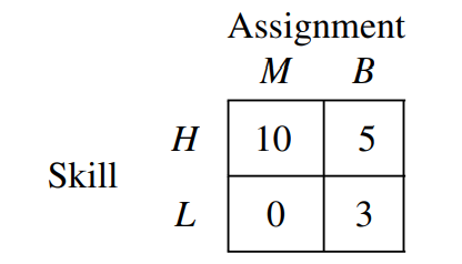
- Player 2 is an employer, who can assign player 1 to one of two jobs. Specifically player 2 can assign player 1 to be either a manager \((M)\) or a blue-collar worker \((B)\), so that his action set is \(A_2=\{M, B\}\). The employer will retain the profit from the project and must pay a wage to the worker depending on the job assignment. The market wage for a manager is \(w_M\) and that for a bluecollar worker is \(w_B\), where \(w_M>w_B\). We assume in particular that \(w_M=10\) and \(w_B=6\).
- Player 2's payoff (the employer's profit) is determined by the combination of skill and job assignments. It is assumed that the MBA degree adds nothing to productivity. A high-skilled worker is relatively better at managing, while a low-skilled worker is relatively better at blue-collar work. The employer's net profits from the possible skill-assignment matches are given in the following table:
Given the information about the game that is laid out in (1)–(4), the complete game tree is represented in Figure 16.1. Because player 2 does not know player 1’s type and only observes his choice, there are two information sets. The two nodes that follow the choice \(U\) are in one information set, and the two nodes that follow the choice \(D\) are in the second information set. In the analysis that follows, we refer to the first information set as \(I_U\) and to the second as \(I_D\).
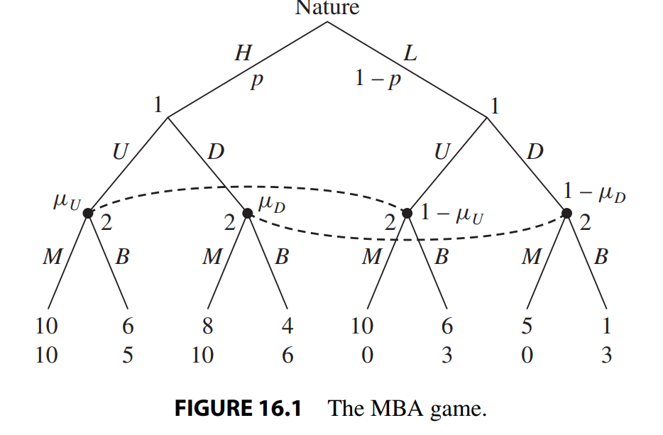
First, to define beliefs, let \(μ_U\) denote the belief of player 2 that player 1’s type is \(H\) conditional on player 1 choosing \(U\), and similarly let \(μ_D\) denote the belief of player2 that player 1’s type is \(H\) conditional on player 1 choosing \(D\). These beliefs will be determined by the distribution of Nature’s choice, together with the beliefs that player 2 holds about the strategy that player 1 is playing. For equilibrium analysis, these beliefs will be determined according to requirements 15.2 and 15.3 described in Section 15.2.
In general if player 1 is using a mixed strategy in which type \(H\) chooses \(U\) with probability \(\sigma^H\) and type \(L\) chooses \(U\) with probability \(\sigma^L\), and if both \(\sigma^H\) and \(\sigma^L\) are strictly between 0 and 1 (i.e., the two types are choosing nondegenerate mixed strategies) then requirement 15.2 implies that by Bayes' rule
and
Notice that if both \(\sigma^H=\sigma^L=1\) (both types are choosing \(U\) ) then beliefs are well defined only by (16.1) from Bayes' rule, so that \(\mu_U=p\), while from (16.2) beliefs are not well defined by Bayes' rule, so we have the freedom to choose \(\mu_D\). Similarly if both \(\sigma^H=\sigma^L=0\) (both types are choosing \(D\) ) then \(\mu_U\) is not well defined while \(\mu_D=p\).
We are now ready to proceed to find the perfect Bayesian equilibria in the MBA game. Because each player has two information sets with two actions in each of these sets, each player has four pure strategies. Let player 1's strategy be denoted \(a_1^H a_1^L\), where \(a_1^\theta \in\{U, D\}\) denotes what player 1 does if he is type \(\theta \in\{H, L\}\). Similarly let \(a_2^U a_2^D\) denote player 2's strategy, where \(a_2^k \in\{M, B\}\) denotes what player 2 does if he observes that player 1 chose \(k \in\{U, D\}\).
To make our analysis more straightforward, assume that Nature chooses player1’s type according to \(p =\frac{1}{4}\), so that we can derive the matrix that is the normalform representation of the MBA Bayesian game. As we have demonstrated earlierfor the entry game, the payoffs in the matrix are calculated by taking each pair of pure strategies, observing which paths are played with the different probabilities that are due to Nature’s choice, and then writing down the derived expected payoffs from this pair of strategies. For example, if \((UD, MB)\) are the pair of strategies then with probability \(\frac{1}{4}\), Nature chooses type \(H\) for player 1 who chooses \(U\), and in response player 2 chooses \(M\), yielding a payoff pair of \((10, 10)\). This follows because player 1 gets a wage of 10 and incurs no cost of obtaining an MBA, while player 2 assigns a high-skill worker to a managerial job, so he obtains a payoff of 10 as well. With probability \(\frac{3}{4}\) Nature chooses type \(L\) for player 1 who chooses \(D\), and in response player 2 chooses \(B\), yielding a payoff pair of \((1, 3)\). This follows because player 1’s net payoff is 6-5 = 1 (wage equal to 6 and a cost of studying equal to 5) and player 2’s net payoff is 3 (assigning a low-skill worker to a blue-collar job). The expected pair of payoffs for the players from the strategy \((UD, MB)\) is therefore $$(v_1,v_2) = 1/ 4 (10, 10) + 3/ 4 (1, 3) = (3.25, 4.75).$$ Similarly we can calculate the expected payoffs for all the other 15 entries in the Bayesian game matrix. Notice that when player 1 plays the same action for the different types (rows 1 and 4) then part of player 2’s strategy is never used, so there are repeat entries which reduce the number of calculations needed. The matrix representation is

If we follow the method of underlining player 1’s best responses for each column and overlining player 2’s best responses for each row, we immediately observe that there are two pure-strategy Bayesian Nash equilibria: \((UU, BB)\) and \((DU, BM)\). To see whether these can be part of a perfect Bayesian equilibrium, we need to find a system of beliefs that support the proposed behavior, and that together with these strategies satisfy requirements 15.1–15.4. From proposition 15.1 it follows that \((DU, BM)\) can be part of a perfect Bayesian equilibrium because all of the information sets are reached with positive probability. In particular the derived beliefs from \((DU, BM)\) are \(μ_U = 0\) and \(μ_D = 1\). It follows from the Bayesian game matrix that player 2 is playing a best response to these beliefs in each of his information sets, and that player 1 is playing a best response in each of his. So \((DU, BM)\) together with \(μ_U = 0\) and \(μ_D = 1\) constitute a perfect Bayesian equilibrium. What about the pair of strategies \((UU, BB)\)? From (16.1) and (16.2), unique beliefs are derived only for information set \(I_U\) because \(I_D\) is reached with zero probability. In particular \(μ_U = 1/4\) and \(μ_D\) is not well defined. It is easy to check that player 2 choosing B is a best response in information set \(I_U\) to the belief \(μ_U = 1/4\). Therefore to see whether \((UU, BB)\) can be part of a perfect Bayesian equilibrium we need to see if there are beliefs μD that support B as a best response for player 2 in information set \(I_D\). For \(B\) to be a best response in the information set \(I_D\), it must be the case that given the belief \(μ_D\) the expected payoff from \(B\) is higher than the expected payoff from M. This can be written down as
which is true if and only if \(μ_D ≤ 3/8\). This implies that we can support \((UU, BB)\) as part of a perfect Bayesian equilibrium. In particular \((UU, BB)\), together with belief \(μ_U = 1/4\) and any belief satisfying \(μ_D ∈ [0, 3/8]\), constitutes a perfect Bayesian equilibrium. We conclude that in the first perfect Bayesian equilibrium with strategies \((DU, BM)\), different types of player 1 choose different actions, thus using their actions to reveal to player 2 their true types. In other words, this is a separating perfect Bayesian equilibrium. In the second perfect Bayesian equilibrium, with strategies \((UU, BB)\), both types of player 1 do the same thing, and thus player 2 learns nothing from player 1’s action; this is a pooling perfect Bayesian equilibrium.